

The Virtual Tumour, part II
Written by David Orrell
As discussed in the last post, models have two functions – to describe, and to predict. In systems biology, and other areas of science, these are often conflated. We say a model is predictive, when really we mean it is descriptive. But prediction – from the Latin praedicere for “make known beforehand” – is not the same as just reproducing something that is already known. The key element here is the “beforehand” part.
As one random example of how the word “predict” tends to be used, there is the paper called “Boolean Network Model Predicts Cell Cycle Sequence of Fission Yeast”. It’s a bit like seeing a headline anouncing “Weather model predicts existence of storms.” It is no use for a model to predict that storms (or cell cycles) exist, we know that already! We want to predict when a storm will exist, and in particular whether it is going to exist above the exact spot where we have planned our outdoor wedding ceremony (or whatever).
My favourite is the physics area of string theory, where an expert once announced: “String theory predicts gravity.” Thanks!
The reason of course why scientists like to claim their models are predictive is that, as Richard Feynman noted, “The test of science is its ability to predict.” So for a theory to be judged as successful, it should be able to make accurate predictions. Conversely, when models fail to make accurate predictions, then in theory that should invalidate them.
In the case of the Virtual Tumour, our aim was to build a model that was predictive, rather than descriptive. And here we come to another issue, which is that description and predicton are not just different, but they are often actually opposed to a degree. Adding extra parameters and more bells and whistles to a model will make it look more realistic. It will also make it less good at prediction, because of the uncertainty around the values for all those parameters, and also how they will interact.
As Gutenkunst et al. wrote in a 2007 paper, the existence of “sloppy parameters” in complex models means that “measurements must be formidably precise and complete to usefully constrain many model predictions.” In practice, the parameters are adjusted to fit the existing data; but because the parameters are under-determined by the data, the result is overfitting. And as Nate Silver pointed out in his 2012 book The Signal and the Noise, “Overfitting represents a double whammy: it makes our model look better on paper but perform worse in the real world.”
This is why, as Makridakis and Hibon (2007) showed, simple models consistently outperform more complicated models at prediction tests. Of course, a model has to capture the essence of the underlying system, so must be what the statistician Arnold Zellner called “sophisticatedly simple”.
Or as the applied mathematican and quantitative finance expert Paul Wilmott puts it, the aim is to operate in the “mathematical sweetspot” between over-simplicity and over-complexity: “Being blinded by mathematical science and consequently believing your models is all too common in quantitative finance” as in systems biology.
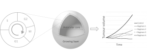
Our approach to this conundrum was to keep the unit of analysis at the level of the cell, but to reduce the complexity of the cell cycle model so that it focused only on the effect of drugs during particular phases. The result was a stripped-down agent-based model which modelled a cell population as the cells grew, divided, were exposed to drugs, and so on – and which could still capture things like synchronisation effects which play such a big role in oncology treatments.
After all, we weren’t trying to predict that tumours exist – we were trying to help stop them. In our next post in this series, we will look at how our approach measures up against other models.